

High blood pressure, or hypertension, affects nearly half of adults in the United States and more than a billion people worldwide. It quietly raises the risk of heart attack, stroke, kidney failure, and other serious problems—often without any warning signs. This guide explains what hypertension is and how blood pressure works. It covers categories and types, symptoms (or lack of them), causes, and risk factors. You will learn how it damages the body, possible complications, and diagnosis. The guide also offers treatment options and natural ways to support lower readings. It discusses prevention strategies, common myths, and provides answers to frequent questions. Everything here draws on established medical understanding from sources like the American Heart Association (AHA), American College of Cardiology (ACC), Centers for Disease Control and Prevention (CDC), and World Health Organization (WHO). What Is Hypertension? Hypertension is the medical term for consistently high blood pressure. Blood pressure measures the force of blood pushing against the walls of your arteries as the heart pumps. When that force stays too high over time, it strains the heart, damages blood vessels, and harms organs. Doctors call hypertension the “silent killer” because most people feel no symptoms until serious damage has already occurred. You can walk around for years with elevated readings and never know it—until a heart attack, stroke, or other crisis appears. Globally, hypertension remains one of the leading preventable causes of death and disability. In the U.S., roughly 48% of adults have high blood pressure (systolic ≥130 mm Hg or diastolic ≥80 mm Hg, or they take medication for it). Many of those people do not have it under control. Early detection matters because the earlier you act—through lifestyle changes or medication when needed—the more you can protect your heart, brain, kidneys, and eyes. How Blood Pressure Works 1. What Is Blood Pressure? Your heart is a powerful pump. With each beat it pushes blood into the arteries. The arteries carry oxygen-rich blood to every part of the body. Blood pressure reflects two forces: the pressure when the heart contracts and the pressure when it relaxes between beats. Healthy arteries are flexible. They stretch slightly with each heartbeat and then return to their normal size. When arteries stiffen or narrow, the same volume of blood creates higher pressure. 2. Systolic vs. Diastolic Blood Pressure A blood pressure reading has two numbers, written as systolic over diastolic (for example, 120/80 mm Hg). Both numbers matter. Elevated systolic pressure is especially important in older adults because arteries naturally stiffen with age. Elevated diastolic pressure can also signal risk, particularly in younger people. Guidelines treat both numbers as clinically significant. 3. How Blood Pressure Is Measured Blood pressure is measured in millimeters of mercury (mm Hg). A healthcare professional or you at home can take the reading with a cuff that inflates around the upper arm. Manual (aneroid) sphygmomanometers use a stethoscope and require training. Digital monitors are widely available, easy to use, and accurate when validated. For best results: Home monitoring gives a more complete picture than occasional clinic visits. Blood Pressure Categories According to the 2025 AHA/ACC guideline, adult blood pressure falls into these categories: Category Systolic (mmHg) Diastolic (mmHg) What It Means Normal Below 120 Below 80 Healthy range; maintain current habits Elevated 120–129 Below 80 Above normal; lifestyle changes recommended Stage 1 Hypertension 130–139 80–89 Mild hypertension; lifestyle changes, possible medication Stage 2 Hypertension 140 or higher 90 or higher Moderate-to-severe; medication usually recommended Hypertensive Crisis Higher than 180 Higher than 120 Medical emergency; seek immediate care A hypertensive crisis requires urgent attention. This is particularly crucial if symptoms like chest pain, shortness of breath, or vision changes occur. Types of Hypertension Not all high blood pressure looks the same. Understanding which type you have shapes how it’s investigated and treated. 1. Primary (Essential) Hypertension This is the most common form, accounting for the vast majority of cases. Primary hypertension develops gradually over years, driven by a mix of genetics, aging, and lifestyle factors, without one single identifiable cause. 2. Secondary Hypertension Secondary hypertension is caused by an underlying, identifiable condition — such as kidney disease, hormonal disorders, or certain medications. It tends to appear more suddenly and can reach higher readings than primary hypertension. Treating the underlying cause often improves or resolves it. 3. Resistant Hypertension This describes blood pressure that remains high despite being on three or more antihypertensive medications, including a diuretic, at optimal doses. It often requires more specialized evaluation to rule out secondary causes or medication issues. 4. White Coat Hypertension Some people have blood pressure readings that spike in a clinical setting due to anxiety about being at the doctor’s office, but are normal elsewhere. This is known as white coat hypertension, and it’s one reason doctors increasingly rely on home or ambulatory monitoring to confirm a diagnosis. 5. Masked Hypertension The opposite of white coat hypertension: blood pressure appears normal in the doctor’s office but is elevated in daily life. Because it’s easy to miss, masked hypertension can be particularly risky if it goes undetected. Type Typical Cause Key Feature Primary (Essential) Multiple factors over time Gradual onset, most common Secondary Identifiable medical condition Sudden onset, often higher readings Resistant Multiple medications, uncontrolled Requires 3+ medications without control White Coat Clinical-setting anxiety High in office, normal elsewhere Masked Situational/lifestyle factors Normal in office, high elsewhere What Causes Hypertension? Hypertension usually results from a combination of factors rather than a single cause. Genetics: A family history of hypertension increases your likelihood of developing it, suggesting inherited factors affect how your body regulates blood pressure. Aging: Arteries naturally stiffen with age, which raises systolic pressure over time even in otherwise healthy people. Obesity: Excess body weight increases the volume of blood your heart must circulate and is linked to hormonal and metabolic changes that raise pressure. Excess salt intake: High sodium consumption causes the body to retain more fluid, increasing blood volume and, in turn, blood pressure. Physical inactivity: A sedentary lifestyle
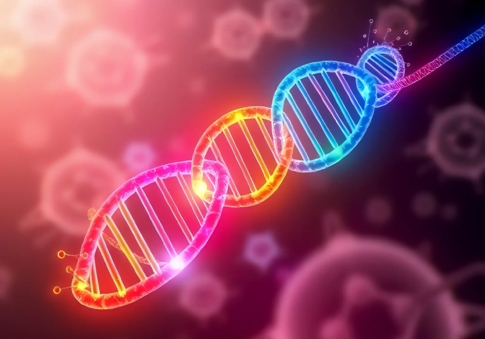
Central Dogma of Life: The One Rule You Must Know About DNA, RNA and Proteins
Biology has a lot of moving parts. Pathways on pathways, weird names, arrows everywhere. But there’s one rule that shows up so often it’s basically the backbone of everything else. If you get this, most “gene” stuff starts to feel… not easy, but at least readable. It’s called the central dogma of life. And yes, it sounds intense. It’s actually pretty simple. What Is the Central Dogma of Life? The central dogma is the core rule for how genetic information usually flows inside cells: DNA → RNA → Protein That’s it. That’s the rule. But here’s the part people miss. This is about information transfer, meaning the sequence. The order of letters in DNA gets copied into RNA, and then that order gets converted into the order of amino acids in a protein. It’s not just “DNA makes proteins.” It’s more like a relay race where the baton is information. A one sentence mental model that actually works: DNA stores the instructions, RNA copies and carries the instructions, proteins do the work. In this article, we’ll walk through the full pipeline, the two big steps that make it happen, and the stuff that gets misunderstood all the time. Gene expression. Transcription. Translation. Why one cell type can act totally different from another even with the same DNA. The usual confusions. Why The Central Dogma of Life Matters: Real-World Examples and Everyday Applications If you ever wonder how a trait happens, like eye color, lactose intolerance, sickle cell disease, muscle growth, height tendencies, whatever. It usually comes back to proteins. Because proteins are what cells use to build and run your body. So the central dogma is basically how your genotype becomes phenotype. Your DNA sequence matters because it affects RNA and proteins, and proteins change what a cell can actually do. You see it in medicine and biotech constantly: Real-Life Example DNA Role RNA Role Protein Role Genetic Testing Detect mutations May alter expression Changes protein function mRNA Vaccines DNA not directly used Delivered mRNA Produces viral protein fragment Antibiotics Target bacterial genes indirectly Target translation process Stop protein production Inherited Diseases Mutated DNA Altered mRNA Defective proteins Practical payoff. If you can follow DNA → RNA → protein, you can follow most headlines that say “Scientists discovered a gene for X.” What they usually mean is “Scientists found a DNA variation that changes a protein, or changes gene expression, and that affects X.” The three main players: DNA, RNA, and proteins Let’s label the cast. DNA Double stranded, long term storage. It’s stable, it lives in the nucleus in eukaryotes, and it holds genes. Think library archive. You do not drag the original manuscript around if you can avoid it. RNA Usually single stranded, more temporary, more flexible. There are multiple types of RNA, and a lot of them do different jobs, but the main one people mean in the central dogma is mRNA (messenger RNA). RNA is the copy, the working document. Proteins Chains of amino acids that fold into specific 3D shapes. And that shape is the whole point. Proteins act as enzymes (speeding up reactions), structural materials, transporters, receptors, signals, motors. They are the “do stuff” molecules. A key bridge idea here is: Sequence → structure → function. DNA and RNA are sequences of nucleotides. Proteins are sequences of amino acids. The amino acid sequence folds into a structure. The structure determines function. That’s how a letter level change in DNA can end up as a body level change in you. Step 1 — DNA: The Source Code of Life and What a Gene Really Is People say “a gene” like it’s one neat chunk of DNA that directly turns into one protein. Real life is messier. A gene often includes: So a gene is not just the protein recipe. It’s also the control panel for that recipe. Also, not all DNA becomes protein. Even within genes, there are parts that won’t end up translated. Plus, huge portions of genomes are regulatory or structural or have functions we are still mapping out. The useful beginner version is: DNA contains both instructions and switches. One more setup concept that matters later: DNA and RNA have direction. You’ll often see 5 prime to 3 prime written as 5’ → 3’. You don’t need the chemistry right now. Just know that copying and reading happen in a consistent direction, like reading a sentence left to right. And finally. Cells do not use the whole genome at once. They are picky. A skin cell expresses skin related genes. A neuron expresses neuron genes. The DNA is mostly the same, the output is different. That leads us to the master idea. Gene Expression in the Central Dogma of Life: How Transcription and Translation Control Protein Synthesis Gene expression is the process of using the information in a gene to make a functional product. Usually that product is a protein. Sometimes it’s a functional RNA (an RNA that does a job directly without becoming a protein). One of the biggest beginner mistakes is confusing: Every cell in your body (with some exceptions like mature red blood cells) has basically the same DNA. But not every cell is making the same RNA or the same proteins. Expression is regulated at multiple stages: Simple example. Liver cells and neurons share the same genome, but they produce different sets of proteins, so they behave like totally different machines. That’s gene expression in action. Now we go through the pipeline. Step 2 — Transcription: how DNA is copied into RNA Transcription is making an RNA copy from a DNA template. The main enzyme is RNA polymerase. Its job is to bind DNA, open a small section, and build an RNA strand by matching bases. At a beginner friendly level, transcription has three stages: One detail that clears up confusion fast: DNA has two strands, but only one is used as the template for a given gene at a given time. You may hear: So the

AI in Wildlife Conservation: How Smart Technology Is Saving Endangered Species in 2026
Wildlife conservation has always been a race. But in 2026 it feels like the track got longer, the weather got worse, and the people running the race are still asked to do it with the same worn-out shoes. At this critical juncture, AI in wildlife conservation is becoming an indispensable ally. With an unprecedented volume of data flooding in—from millions of camera trap images and thousands of hours of forest audio to satellite updates, drone surveys, ranger notes, and community reports—human teams alone cannot keep up. AI is not a magic fix for biodiversity loss. But it is starting to do something that matters a ton in the real world: it turns overwhelming streams of messy conservation data into usable decisions faster. Sometimes fast enough to prevent damage instead of just documenting it later. Why wildlife conservation needs AI now (and why 2026 feels different) The pressures are stacking up. Habitat loss is still moving fast, especially around roads, farms, mining, and expanding settlements. Climate change is pushing range shifts in a way that makes “protected area boundaries” feel kind of… old fashioned. Wildlife crime is adaptive and organized. And most field teams are chronically underfunded, understaffed, and expected to cover absurdly large landscapes. So what is different by 2026? A bunch of practical things changed at once: Reader promise, plainly: this article is about the practical ways AI is being used in 2026 to detect threats earlier, monitor populations more accurately, and stretch limited conservation budgets. And one boundary that matters. AI supports field teams. It does not replace ecological expertise, Indigenous and community-led stewardship, or the political work of protecting land and water. If someone sells it that way, that is usually a warning sign. What “AI in wildlife conservation” actually means (in plain English) When people say “AI for conservation,” they usually mean a stack of three things: 1) Data collection Where the raw signals come from: 2) Modeling Machine learning models that turn raw signals into predictions, like: Here, it’s important to note that adversarial machine learning, a subfield of machine learning, can also play a role in enhancing these predictive models by making them more robust against adversarial inputs. 3) Action Where it becomes conservation, not just analytics: A few quick glossary-style clarifications: The important part is mapping outputs to decisions. AI can produce: Also, field reality: good enough + fast often beats perfect + slow. If an acoustic sensor flags a likely chainsaw event with 85 percent confidence and rangers can respond within hours, that may save more forest than a 99 percent perfect model that delivers results two weeks later. In addition to these practical applications, it’s also worth noting that AI’s role in wildlife conservation extends beyond just data analysis and action. It can also be utilized as an educational tool. For instance, platforms offering science quizzes can help raise awareness about wildlife conservation issues by providing interactive learning experiences. The core conservation problems AI is helping solve This is the simplest way I know to explain why AI is showing up everywhere in conservation now. The monitoring problem Counting animals is expensive, slow, and often invasive. AI speeds up identification, reduces manual review, and helps detect trends earlier. The detection problem Illegal logging and poaching often go unnoticed until after the fact. AI can flag anomalies from sound, imagery, and movement patterns so teams can respond sooner. The prioritization problem Rangers and funds are limited. AI helps allocate patrols, cameras, and restoration work where it is most likely to matter. The evaluation problem A painful truth: lots of interventions are not measured well. AI makes before/after comparisons across large areas more feasible, so projects can learn and adapt instead of repeating habits. AI animal tracking in 2026: from collars to computer vision “Tracking” used to mostly mean collars. And collars are still hugely important for some questions, especially movement ecology and human-wildlife conflict. But by 2026 tracking is a bigger menu: Where AI changes the game is reducing manual labor: And a big 2026 shift: edge AI. Instead of transmitting everything, some camera traps and acoustic devices can run lightweight models on-device to: That means less battery drain, less bandwidth cost, and fewer “we collected data but can’t move it” failures. Trade-offs still exist: A concrete example flow (what this looks like in practice): Camera trap → AI filters empty frames → species or individual ID → dashboard trendline and map → ranger or biologist action (move cameras, target patrols, anti-snare sweep, corridor planning) The success of these AI applications largely hinges on effective MLOps, which involves deploying and maintaining AI models with a scientific approach. Camera traps + computer vision: the biggest time-saver Camera traps create a weird kind of suffering for conservation teams. Not the cameras themselves. The folders. Endless folders. Computer vision models typically do three things: Individual re-ID is where things get really interesting for certain species. Tigers, leopards, zebras, giraffes, whale sharks. Anything with consistent patterns or markings. This is where Named Entity Recognition comes into play. It helps AI systems to not only identify individual animals but also understand their unique characteristics better. Why it matters: population estimates and survival rates often depend on identifying individuals over time. If AI can reliably match individuals, it accelerates mark-recapture style analyses and reduces human error from fatigue. Humans stay in the loop, ideally like this: Practical tips (because these are the boring things that determine success): Drones + thermal imaging: fast surveys with fewer blind spots Drones are not a replacement for boots on the ground, but they can compress time. Common use cases: Thermal helps because heat signatures show up in low light. But thermal is not magic either. Limitations: Operational reality matters: AI helps by: Satellites + AI: protecting habitats at scale Satellites are the only practical way to monitor huge areas consistently. They are not perfect, but they are relentless. Remote sensing basics, in normal language: Use cases: “Near real time” in practice depends on
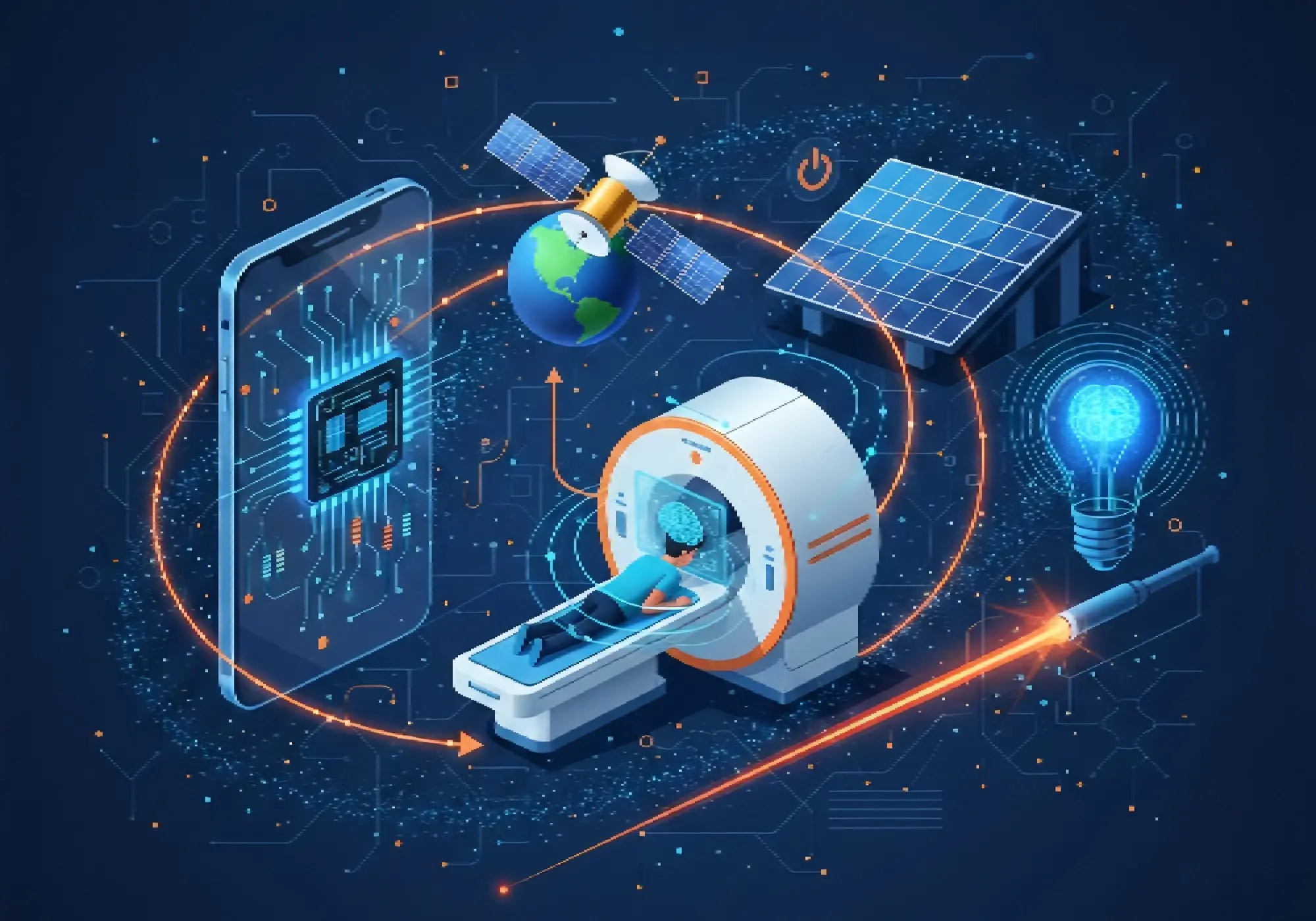
Applications of Modern Physics in Everyday Life: From Lasers to GPS, MRI & Beyond
Every time you check your phone’s location, step into a hospital for a scan, or switch on an LED light, you’re seeing applications of modern physics. It may feel normal. However, behind these simple actions lies one of the greatest scientific revolutions in history. Modern physics was born in the early 20th century. At first, it sounded abstract and even strange. Scientists talked about quantum mechanics and relativity—ideas that bent the rules of classical physics. Yet over time, those bold theories turned into the backbone of today’s technology. Now they power the devices we use every single day. So, what exactly is modern physics? In simple terms, it studies matter, energy, space, and time at extreme scales. When Newton’s laws stop working, modern physics steps in. It explains the behavior of tiny particles through quantum mechanics. It also explains fast-moving objects and massive bodies through relativity. In addition, it deepens our understanding of electromagnetic radiation. These concepts are not just classroom topics. Instead, they drive GPS systems, medical imaging tools, powerful computers, and countless real-world technologies. That’s why understanding these everyday applications truly matters. Technology is evolving fast. Quantum computers are emerging. Advanced sensors are becoming smarter. AI-based medical tools are growing more accurate. As a result, knowing the physics behind these innovations helps us see the bigger picture. It allows us to appreciate not only what exists today but also what is coming next. From the lasers inside a Blu-ray player to atomic clocks that keep global communication in sync, modern physics is everywhere. It is not locked inside research labs. Rather, it lives in your pocket, sits on your wrist, and surrounds you at every moment. Core Principles of Modern Physics Explained Simply for Beginners Before diving into specific technologies, let’s understand the three fundamental pillars of modern physics that make today’s innovations possible. 1. Quantum Mechanics Basics Quantum mechanics, explained in simple terms, uncovers a surprising truth: at the atomic and subatomic level, the world doesn’t follow the rules we see around us every day. Instead of moving like tiny solid balls, particles act in strange and unexpected ways. They don’t have fixed positions or clear speeds. Instead, they exist as probabilities — possibilities — until we actually measure them. For example, electrons don’t travel around the nucleus in neat circular paths like planets around the Sun. Rather, they exist in “clouds” of probability. These clouds show where an electron is most likely to be found when we observe it. Key quantum concepts that enable modern technology include: These principles aren’t philosophical abstractions. They’re the reason semiconductors work, lasers emit coherent light, and MRI machines can image soft tissue inside your body. 2. Relativity Fundamentals Einstein completely changed how we see the universe. His theories of relativity reshaped our understanding of space, time, and gravity forever. First came special relativity in 1905. It showed something mind-blowing: space and time are not separate. They are connected. Even more surprising, time does not move the same for everyone. When something travels very fast, its clock slows down. This effect is called time dilation. So in simple terms, the faster you move, the slower time passes for you. Then, in 1915, Einstein introduced general relativity. This theory went deeper. It explained gravity in a totally new way. Instead of thinking of gravity as a force pulling objects together, Einstein described it as a bending of spacetime. Massive objects like planets and stars curve the fabric of spacetime around them. As a result, other objects move along those curves. That curved motion is what we experience as gravity. Now here’s the exciting part. Relativity is not just theory. It powers modern technology. Take GPS systems, for example. Satellites orbit Earth at very high speeds. At the same time, they are farther from Earth’s gravity compared to us on the ground. Because of their speed, special relativity makes their clocks run slightly slower. However, because they experience weaker gravity, general relativity makes their clocks run slightly faster. Both effects happen together. If scientists did not correct these tiny time differences, GPS would drift off by several kilometers each day. Navigation would fail. Maps would be unreliable. In short, modern location services would not work. So next time you open Google Maps, remember: you are using Einstein’s relativity in real time. 3. Electromagnetism and Wave-Particle Ideas The electromagnetic (EM) spectrum uses span from radio waves to gamma rays, all traveling at the speed of light but with vastly different energies and wavelengths. Modern physics revealed that electromagnetic radiation behaves as both continuous waves and discrete particles called photons. This dual nature enables: Understanding how photons interact with electrons in materials opened the door to semiconductor physics, photonics and optics, and the entire digital revolution. Everyday Applications of Modern Physics in Daily Life Modern physics isn’t just theory sitting in textbooks. It drives the technology you use every single day. So instead of thinking of it as abstract science, think of it as the hidden engine behind your daily life. From the moment you wake up, it’s already at work. Now, let’s break it down and explore the real-world physics innovations behind the devices you probably used today. Lasers: How Stimulated Emission Enables Technology The word “laser” stands for Light Amplification by Stimulated Emission of Radiation, and this process is pure quantum mechanics in action. In a laser, atoms are excited to higher energy states, then stimulated to release photons in a coordinated way, producing an intense, coherent beam of light. Laser everyday uses include: The key advantage? Lasers produce monochromatic (single-color) light that can be focused to incredibly small spots, delivering precise energy exactly where needed. This quantum phenomenon transformed medicine, manufacturing, and communication. GPS: Relativity and Timekeeping Precision Your smartphone can pinpoint your location within meters anywhere on Earth, thanks to a constellation of 24+ satellites orbiting 20,000 kilometers above. But this everyday miracle depends critically on understanding GPS time dilation. Here’s how it works: Each GPS satellite broadcasts precise time